Ridge, lasso, and elastic net regression
Categories:
Reference
[ESL] Trevor Hastie, Robert Tibshirani, and Jerome Friedman. The Elements of Statistical Learning (second edition) (2009).
https://hastie.su.domains/ElemStatLearn/
https://link.springer.com/book/10.1007%2F978-0-387-84858-7
Section 2.3, 3.1, 3.2, 3.4, 4.4
Linear models and least squares
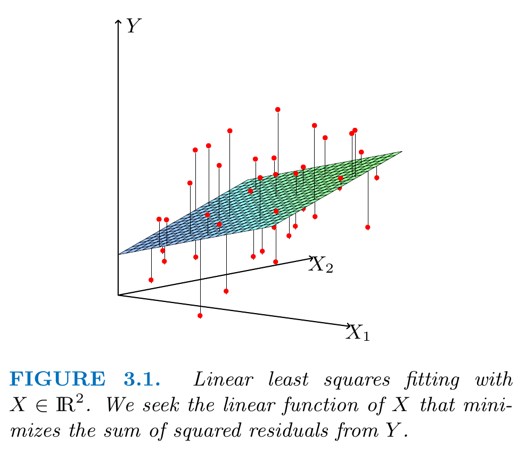
In a linear model, a (continuous) output \(Y\) is predicted from a vector of inputs \(X^T=(X_1,X_2,\dots,X_p)\) via $$\begin{aligned} \hat Y = \hat\beta_0 + \sum_{j=1}^p \hat{\beta}_j X_j \end{aligned}$$
- \(\hat Y\) is the predicted value of \(Y\),
- \(\hat\beta_0\) is the intercept (in statistics) or bias (in machinelearning),
- \((\hat\beta_1,\hat\beta_2,\dots,\hat\beta_p)^T\) is the vector of (regression) coefficients,
For convenience, we often include a constant variable 1 in $X$, include $\hat \beta_0$ in the vector of coefficients, and write the linear model in vector form: $$\begin{aligned} \hat Y = X^T\hat\beta \end{aligned}$$
Least squares is the most popular method to fit the linear model to a set of training data $(x_1,y_1)$ $\dots$ $(x_N,y_N)$: we pick the coefficients $\beta$ to minimize the residual sum of squares
$$\begin{aligned} RSS(\beta) &= \sum_{i=1}^N (y_i - \hat y_i)^2 = \sum_{i=1}^N \left(y_i - x_i^T\beta\right)^2 = \sum_{i=1}^N \Bigl(y_i - \sum_{j=1}^p x_{ij}\beta_j\Bigr)^2 \end{aligned}$$
Collecting the data for the inputs and ouptput in a $N\times p$ matrix $\mathbf{X}$ and $N$-vector $\mathbf{y}$, respectively, $$\begin{aligned} \mathbf{X}= (x_1,x_2,\dots,x_p) = \begin{pmatrix} x_{11} & x_{12} & \dots & x_{1p}\\ x_{21} & x_{22} & \dots & x_{2p}\\ \vdots & \vdots & & \vdots\\ x_{N1} & x_{N2} & \dots & x_{Np} \end{pmatrix} && \mathbf{y}= \begin{pmatrix} y_1\\ y_2\\ \vdots\\ y_N \end{pmatrix} \end{aligned}$$ we can write $$\begin{aligned} RSS(\beta) &= (\mathbf{y}-\mathbf{X}\beta)^T(\mathbf{y}-\mathbf{X}\beta) \end{aligned}$$ If the $p\times p$ matrix $\mathbf{X}^T\mathbf{X}$ is non-singular, then the unique minimizer of $RSS(\beta)$ is given by $$\tag{1} \hat\beta = (\mathbf{X}^T\mathbf{X})^{-1} \mathbf{X}^T\mathbf{y}$$
Exercise
Prove eq. (1) by differentiating $RSS(\beta)$ w.r.t. $\beta_i$.The fitted value at the $i$th input $x_i$ is $\hat y_i=x_i^T\hat\beta$. In matrix-vector notation, we can write $$\begin{aligned} \hat{\mathbf{y}} = \mathbf{X}\hat\beta = \mathbf{X}(\mathbf{X}^T\mathbf{X})^{-1}\mathbf{X}^T\mathbf{y} \end{aligned}$$ Write $$\begin{aligned} \mathbf{H}= \mathbf{X}(\mathbf{X}^T\mathbf{X})^{-1}\mathbf{X}^T \end{aligned}$$
Exercise
Show that $\mathbf{H}$ is a projection matrix, $\mathbf{H}^2=\mathbf{H}$. $\mathbf{H}$ projects on the linear subspace of $\mathbb{R}^N$ spanned by the columns of $\mathbf{X}$.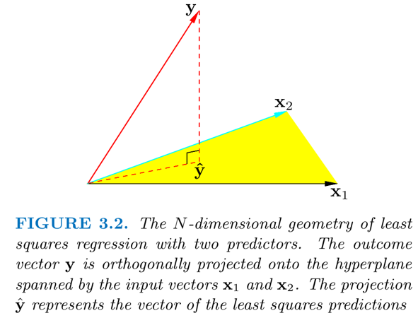
Limitations of least-squares linear regression
Least-squares linear regression involves the matrix inverse $(\mathbf{X}^T\mathbf{X})^{-1}$:
- If the columns of $\mathbf{X}$ are not linearly independent ($\mathbf{X}$ is not full rank), then $\mathbf{X}^T\mathbf{X}$ is singular and $\hat\beta$ are not uniquely defined, although the fitted values $\hat{\mathbf{y}}=\mathbf{X}\hat\beta$ are still the projection of $\mathbf{y}$ on the column space of $\mathbf{X}$. This is usually resolved automatically by stats software packages.
- If $\mathbf{X}$ is full rank, but some predictors are highly correlated, $\det(\mathbf{X})$ will be close to 0. This leads to numerical instability and high variance in $\hat\beta$ (small changes in the training data lead to large changes in $\hat\beta$).
- If $p>N$ (but $rnk(\mathbf{X})=N$), then the columns of $\mathbf{X}$ span the entire space $\mathbb{R}^N$, that is, $\mathbf{H}=\mathbb{1}$ and $\hat{\mathbf{y}}=\mathbf{y}$: overfitting the training data.
High variance and overfitting result in poor prediction accuracy (generalization to unseen data).
Prediction accuracy can be improved by shrinking regression coefficients towards zero (imposing a penalty on their size).
Ridge regression
Regularization by shrinkage: Ridge regression
The ridge regression coefficients minimize a penalized residual sum of of squares: $$\tag{2} \beta^{\text{ridge}} = \argmin_\beta \left\{ \sum_{i=1}^N \Bigl(y_i - \beta_0 - \sum_{j=1}^p x_{ij}\beta_j\Bigr)^2 + \textcolor{red}{\lambda\sum_{j=1}^p\beta_j^2} \right\} $$
- $\lambda\geq 0$ is a hyperparameter that controls the amount of shrinkage.
- The inputs $X_j$ (columns of $\mathbf{X}$) are normally standardized before solving eq. (2).
- The intercept $\beta_0$ is not penalized.
- With centered inputs, $\hat\beta_0=\bar y=\frac1N\sum_i y_i$, and remaining $\beta_j$ can be estimated by a ridge regression without intercept.
The criterion in eq. (2) can be written in matrix form: $$\begin{aligned} RSS(\beta,\lambda) = (\mathbf{y}-\mathbf{X}\beta)^T(\mathbf{y}-\mathbf{X}\beta) + \lambda \beta^T\beta \end{aligned}$$ with unique minimizer $$\tag{3} \beta^{\text{ridge}}= (\mathbf{X}^T\mathbf{X}+\lambda\mathbb{1})^{-1}\mathbf{X}^T\mathbf{y}$$
Note that $\mathbf{X}^T\mathbf{X}+\lambda\mathbb{1}$ is always non-singular.
Exercise
Prove eq. (3) by differentiating $RSS(\beta)$ w.r.t. $\beta_i$Lasso regression
Lasso regression: regularization by shrinkage and subset selection
The lasso regression coefficients minimize a penalized residual sum of squares: $$\tag{4} \beta^{\text{lasso}}= = \argmin_\beta \left\{ \sum_{i=1}^N \Bigl(y_i - \beta_0 - \sum_{j=1}^p x_{ij}\beta_j\Bigr)^2 + \textcolor{red}{\lambda\sum_{j=1}^p|\beta_j|} \right\}$$
- Lasso regression has no closed form solution, the solutions are non-linear in the $y_i$,
- If $\lambda$ is large enough, some coefficients will be exactly zero.
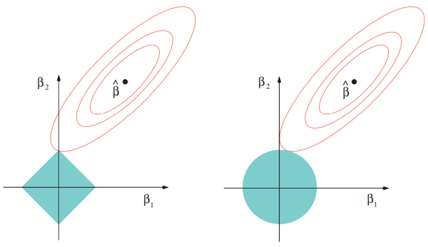
Estimation picture for the lasso (left) and ridge regression (right). Shown are contours of the least squares error (red) and constraint (blue) functions.
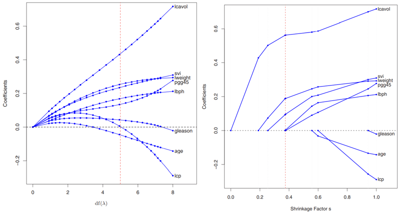
Profiles of ridge (left) and lasso (right) coefficients as the penalty paramater $\lambda$ is varied.
Exercise
Consider the case with one predictor ($p=1$) and training data $$\begin{aligned} \mathbf{x}= \begin{pmatrix} x_1\\ x_2\\ \vdots\\ x_N \end{pmatrix} && \mathbf{y}= \begin{pmatrix} y_1\\ y_2\\ \vdots\\ y_N \end{pmatrix} \end{aligned}$$ Assume that the data are standardized (mean zero and standard deviation one), and that $\mathbf{x}^T\mathbf{y}>0$ (positive correlation between input and output).
- Write down the loss functions and find analytic solutions for the ordinary least squares, ridge regression, and lasso regression coefficient.
- Draw schematically how $\beta^{\text{ridge}}$ and $\beta^{\text{lasso}}$ vary as a function of $\beta^{\text{OLS}}$.
- Explain what shrinkage and variable selection mean in this simple example.
How can the exact lasso solution with one predictor be used to construct an algorithm to solve the general case?
Elastic net regression
Elastic net regression combines ridge and lasso regularization.
- In genomic applications, there are often strong correlations among predictor variables (genes operate in molecular pathways).
- The lasso penalty is somewhat indifferent to the choice among a set of strong but correlated variables.
- The ridge penalty tends to shrink the coefficients of correlated variables towards each other.
- The elastic net penalty is a compromise, and has the form $$\begin{aligned} \lambda\sum_{j=1}^p \Bigl(\alpha|\beta_j|+\tfrac12(1-\alpha)\beta_j^2\Bigr). \end{aligned}$$ The second term encourages highly correlated features to be averaged, while the first term encourages a sparse solution in the coefficients of these averaged features.
Generalized linear models
- Ridge, lasso, and elastic net regression can also be used to fit generalized linear models when the number of predictors is high.
- The most commonly used model is logistic regression, where a binary output $Y$ is predicted from a vector of inputs $X^T=(X_1,\dots,X_p)$ via $$\begin{aligned} \log\frac{P(Y=1\mid X)}{P(Y=0\mid X)} &= \beta_0 + \sum_{j=1}^p \beta_j X_j\\ P(Y=1\mid X) = 1 - P(Y=0\mid X) &= \frac1{1+e^{-\beta_0 - \sum_{j=1}^p \beta_j X_j}} \end{aligned}$$
- With training data $(\mathbf{X},\mathbf{y})$, the parameters are estimated by maximizing the penalized log-likelihood: $$\begin{aligned} \mathcal{L}(\beta) &= \log \prod_{i=1}^N P(y_i\mid x_{i1},\dots,x_{ip}) - \sum_{j=1}^p \left(\alpha|\beta_j|+\tfrac12(1-\alpha)\beta_j^2\right)\\ &= \sum_{i=1}^N \log P(y_i\mid x_{i1},\dots,x_{ip}) - \lambda \sum_{j=1}^p \left(\alpha|\beta_j|+\tfrac12(1-\alpha)\beta_j^2\right) \end{aligned}$$
- Generalized linear models can be fitted using a iterative least squares approximation: a quadratic approximation to the log-likelihood around the current estimates for $\beta$, and this quadratic approximation is used to find the next estimates using the standard linear elastic net solution.
Exercise
Find an expression for $\L(\beta)$ in the case of logistic regression.Bayesian regularized regression
Assignment
CCLE data analysis
We will use data from the original Cancer Cell Line Encyclopedia.
https://www.nature.com/articles/nature11003
Download and import data:
- Expression data from GSE36139; use the Series Matrix File GSE36139-GPL15308_series_matrix.txt
- Drug sensitivities: Supplementary Table 11 from the original publication; use the “activitiy area” (actarea) as a response variable.
Clean data:
- Remove genes with low standard deviation
- Remove compounds with more than 10% zero values
- Align gene expression and sensitivity data to a common set of samples
Find and understand, and implement the elastic net regression fitting procedure employed by the authors in the paper’s supplementary methods. Efficient implementations for fitting ridge, lasso, and elastic net regularized regression models are available in most programming languages (R, python, julia, matlab), search for glmnet in your language of choice!
Reproduce Fig 2c and Fig 4a. Do you find the same selected expression features? Note that the paper used both gene expression and mutational features and you used only gene expression features. How could this difference affect the results?