Bayesian networks
Categories:
Reference
Friedman, Inferring Cellular Networks Using Probabilistic Graphical Models
Christopher Bishop. Pattern Recognition and Machine Learning (2006). Chapter 8
Inferring Cellular Networks Using Probabilistic Graphical Models
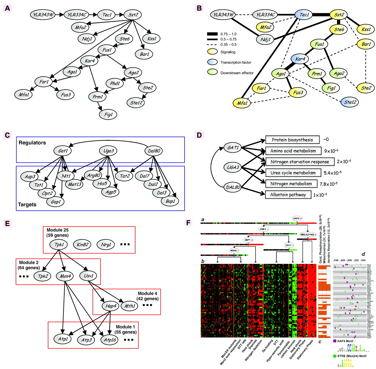
Figure 1
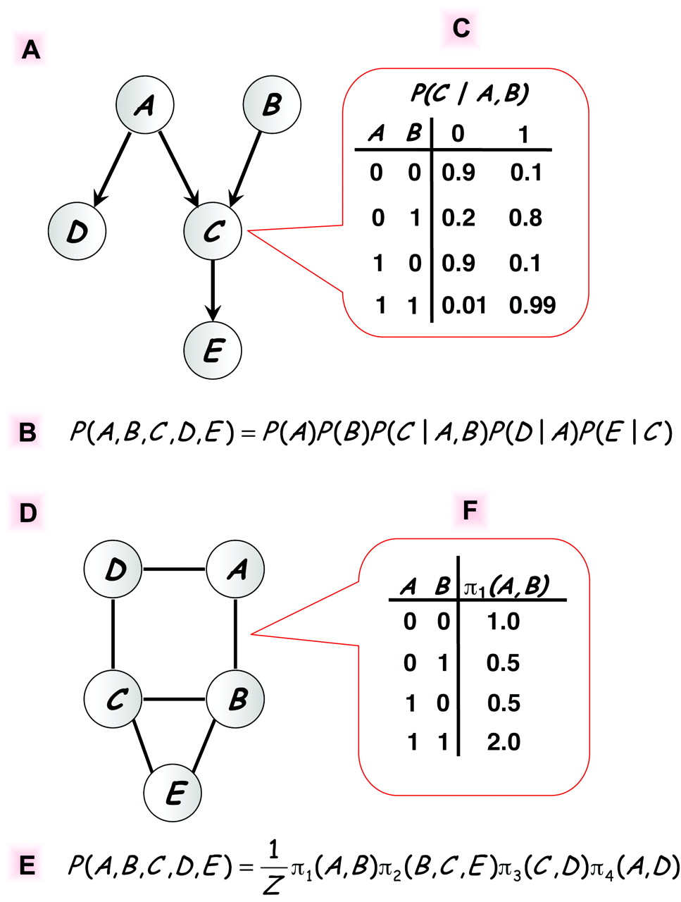
Figure 3
A crash course in Bayesian networks
In Bayesian networks, the joint distribution over a set ${X_1,\dots, X_p}$ of random variables is represented by:
- a directed acyclic graph (DAG) $\cal G$ with the variables as vertices,
- a set of conditional probability distributions, $$\begin{aligned} P\bigl(X_i \mid {X_j \mid j\in \mathrm{Pa}_i}\bigr), \end{aligned}$$ where $\mathrm{Pa}_i$ is the set of parents of vertex $i$ in $\mathcal{G}$,
such that $$\begin{aligned} P(X_1,\dots,X_p) = \prod_{i=1}^p P\bigl(X_i \mid {X_j \mid j\in \mathrm{Pa}_i}\bigr) \end{aligned}$$
In GRN reconstruction:
- $X_i$ represents the expression level of gene $i$,
- $P(X_1,\dots,X_p)$ represents the joint distribution from which (independent) experimental samples are drawn,
- $\mathcal{G}$ represents the unknown GRN.
Assume we have a set of $N$ observations $x_1,\dots,x_N\in \mathbb{R}^p$ of $p$ variables, collected in the $N\times p$ matrix $\mathbf{X}$.
Assume we know $\mathcal{G}$ and the conditional distributions. Then the likelihood of observing the data is:
$$\begin{aligned} P(\mathbf{X}\mid \mathcal{G}) &= \prod_{k=1}^N P(X_{k1},\dots,X_{kp}\mid \mathcal{G})\\ &= \prod_{i=1}^p \prod_{k=1}^N P\bigl(X_{ki} \mid {X_{kj} \mid j\in \mathrm{Pa}_i}\bigr) \end{aligned}$$
We can now use an iterative algorithm to optimize $\mathcal{G}$ and the conditional distributions:
- Start with a random graph $\mathcal{G}$.
- Given $\mathcal{G}$, the likelihood decomposes in a product of independent likelihoods, one for each gene, and the conditional distributions can be optimized by standard regression analysis.
- In the next iterations, randomly add, delete, or reverse edges in $\mathcal{G}$, as long as the likelihood improves.
A more formal approach to optimizing $\mathcal{G}$ uses Bayes’ theorem: $$\begin{aligned} P(\mathcal{G}\mid \mathbf{X}) = \frac{P(\mathbf{X}\mid \mathcal{G}) P(\mathcal{G})}{P(\mathbf{X})} \end{aligned}$$
- $P(\mathcal{G})$ represents the prior distribution: even without seeing any data, not all graphs need to be equally likely a priori.
- $P(\mathbf{X})$ represents the marginal distribution: $P(\mathbf{X}) = \sum_{\mathcal{G}’} P(\mathbf{X}\mid \mathcal{G}’) P(\mathcal{G}’)$. It is independent of $\mathcal{G}$ and can be ignored.
We can use $P(\mathcal{G})$ to encode evidence for causal interactions from integrating genomics and transcriptomics data. This is the main idea from Zhu et al. (2004).